
A single reversed formula can turn a straightforward PMP calculation into a costly exam mistake. This PMP formula cheat sheet covers earned value management (EVM), PERT estimates, critical path calculations, Agile delivery metrics, forecasting, and financial decision formulas with worked examples and interpretation rules. Built around the PMP examination framework introduced in July 2026, it helps candidates preparing for 2027–2028 recognize the correct calculation, avoid common traps, and connect numerical results to project decisions. Use it alongside PMP exam preparation resources, exam domain guidance, and common exam mistakes.

1. Which PMP Formulas Matter Most for the 2027–2028 Exam?
The July 2026 PMP exam update established three domain weights: People (33%), Process (41%), and Business Environment (26%). Approximately 40% of the exam represents predictive project management, while the remaining 60% is divided between Agile/adaptive and hybrid approaches. This remains the latest published framework as of November 2026; candidates sitting in 2027 or 2028 should confirm PMI's applicable exam outline before testing.
Formula preparation should therefore support business decisions across delivery approaches. The strongest candidates can calculate a performance indicator, interpret its consequences, and identify the next responsible project management action.
For example, a CPI of 0.80 indicates that the project earns only $0.80 of budgeted value for every $1.00 spent. That number becomes useful when it informs a revised forecast, corrective action, or stakeholder discussion.
This is why earned value calculations, PMP exam domain analysis, exam preparation techniques, and decision-oriented mock practice belong together.
Learn Formulas in Five Priority Groups
Priority 1: Earned value and cost forecasting. Understand PV, EV, AC, BAC, CV, SV, CPI, SPI, EAC, ETC, VAC, and TCPI. These formulas test the ability to judge current performance and forecast the financial consequences of remaining work.
Priority 2: Scheduling and estimation. Know PERT, triangular estimates, standard deviation, activity variance, float, and critical path logic. Focus on how uncertainty and dependencies influence schedule commitments.
Priority 3: Agile flow and capacity. Understand velocity, throughput, lead time, cycle time, work in progress, burndown, and Little's Law. These support Agile project management, scaled Agile delivery, and Scrum@Scale coordination.
Priority 4: Risk and financial evaluation. Practice expected monetary value, return on investment, net present value, benefit-cost ratio, and payback period. These help evaluate alternatives and support project governance decisions.
Priority 5: Resource and communication calculations. Understand communication channels, resource utilization, capacity, and productivity ratios. These are useful when analyzing stakeholder responsibilities, program coordination, and project performance data.
How to Read Formula Questions Correctly
Before calculating, identify what the question is asking:
Current performance: CPI, SPI, CV, or SV.
Total expected final cost: EAC.
Cost of unfinished work: ETC.
Expected final budget difference: VAC.
Efficiency required to meet a target: TCPI.
Expected duration under uncertainty: PERT.
Schedule flexibility: Total float.
Expected financial exposure: EMV.
Time required to finish an Agile backlog: Velocity- or throughput-based forecasting, depending on the unit of work.
A question asking for the cost of remaining work needs ETC, while one asking for the forecast total project cost needs EAC. This distinction regularly appears in EVM calculator practice and is a valuable focus for PMP exam preparation.
| Formula / Metric | Calculation | How to Interpret It | Common Exam Trap |
|---|---|---|---|
| 1. CV Cost Variance | EV − AC | Positive = under budget; negative = over budget. | Reversing EV and AC. |
| 2. SV Schedule Variance | EV − PV | Positive = ahead; negative = behind, in budget-value terms. | Reading SV as a number of days. |
| 3. CPI Cost Performance Index | EV / AC | Above 1 = cost efficient; below 1 = inefficient. | Assuming a higher actual cost improves CPI. |
| 4. SPI Schedule Performance Index | EV / PV | Above 1 = ahead of baseline; below 1 = behind. | Using AC instead of PV. |
| 5. PV Planned Value | BAC × planned completion fraction | Budgeted value of work scheduled by the status date. | Using actual completion. |
| 6. EV Earned Value | BAC × actual earned completion fraction | Budgeted value of work actually accomplished. | Equating EV with money spent. |
| 7. BAC Budget at Completion | Sum of authorized budgeted work | Total approved performance-measurement budget. | Confusing BAC with revised EAC. |
| 8. EAC Typical CPI Forecast | BAC / CPI | Forecast final cost if current cost efficiency continues. | Applying this when future work is expected to perform differently. |
| 9. EAC Bottom-Up Forecast | AC + revised ETC | Forecast using a fresh estimate of unfinished work. | Treating ETC as BAC − EV without verifying assumptions. |
| 10. EAC Original Remaining Budget | AC + (BAC − EV) | Assumes future remaining work performs at planned cost. | Using this when past inefficiency is expected to continue. |
| 11. EAC Cost & Schedule Forecast | AC + (BAC − EV) / (CPI × SPI) | Scenario forecast when both indices are assumed to affect remaining cost. | Applying the model without the scenario's assumptions. |
| 12. ETC Estimate to Complete | EAC − AC | Forecast cost of remaining work. | Confusing remaining cost with total final cost. |
| 13. VAC Variance at Completion | BAC − EAC | Positive = forecast under budget; negative = overrun. | Reversing the subtraction. |
| 14. TCPI Target BAC | (BAC − EV) / (BAC − AC) | Required remaining cost efficiency to achieve BAC. | Using BAC target when it has been replaced. |
| 15. TCPI Target EAC | (BAC − EV) / (EAC − AC) | Required remaining cost efficiency to achieve a specified EAC. | Using the BAC denominator instead. |
| 16. PERT Weighted Mean | (O + 4M + P) / 6 | Expected duration using optimistic, most likely and pessimistic estimates. | Forgetting four times the most likely value. |
| 17. Triangular Estimate | (O + M + P) / 3 | Unweighted mean of three estimates. | Confusing it with PERT. |
| 18. PERT σ Standard Deviation | (P − O) / 6 | Approximate activity-duration uncertainty. | Confusing standard deviation with variance. |
| 19. PERT Variance | [(P − O) / 6]² | Squared dispersion measure for activity duration. | Adding standard deviations directly across a path. |
| 20. Path σ | √(sum of activity variances) | Approximate path uncertainty under independence assumptions. | Ignoring correlations between activities. |
| 21. Total Float | LS − ES or LF − EF | Delay allowance before the project finish is affected. | Assuming a negative value means spare time. |
| 22. Free Float | Earliest successor ES − current EF | Delay allowance without delaying an immediate successor's early start. | Confusing free float with total float. |
| 23. EMV Expected Monetary Value | Probability × monetary impact | Probability-weighted gain or loss. | Dropping the negative sign for losses. |
| 24. Communication Channels | n(n − 1) / 2 | Potential pairwise channels among n participants. | Using n² or counting the same pair twice. |
| 25. ROI Return on Investment | (Net benefit / investment cost) × 100% | Percentage return on invested cost. | Using gross benefits where net benefit is required. |
| 26. BCR Benefit-Cost Ratio | Present value of benefits / present value of costs | Above 1 suggests benefits exceed costs. | Mixing discounted and undiscounted values. |
| 27. NPV Net Present Value | Σ CFₜ / (1 + r)ᵗ − initial investment | Net value today of forecast future cash flows. | Ignoring when each cash flow occurs. |
| 28. Payback Simple Payback | Initial investment / equal annual net cash inflow | Time to recover initial capital with uniform inflows. | Using this shortcut for uneven cash flows. |
| 29. Velocity | Accepted story points / iteration | Historical delivery capacity in team-specific points. | Comparing velocity across unrelated teams. |
| 30. Iterations Remaining | Remaining story points / forecast velocity | Approximate iterations needed; round upward for full iterations. | Assuming velocity is constant. |
| 31. Throughput | Completed work items / time period | Delivery frequency using a consistently defined item. | Mixing item sizes or counting unfinished items. |
| 32. Cycle Time | Completion time − work start time | Elapsed time from starting work to finishing it. | Including pre-start queue time when measuring cycle time. |
| 33. Lead Time | Delivery time − request entry time | Customer-facing elapsed time from request to delivery. | Confusing customer lead time with cycle time. |
| 34. Little's Law | WIP = throughput × average time in system | Relates inventory, throughput and flow time in a stable system. | Using inconsistent system boundaries or an unstable flow. |
| 35. Resource Utilization | Used capacity / available capacity × 100% | Fraction of resource capacity consumed. | Assuming 100% utilization maximizes flow efficiency. |
| 36. Defect Density | Confirmed defects / measured output size | Defect frequency per defined unit. | Comparing projects with different units or reporting rules. |
2. How Do You Solve PMP Earned Value Management (EVM) Questions?
EVM integrates completed work, planned work, and actual expenditure. Most calculation mistakes happen because candidates confuse these three inputs before applying the formula.
Think of them as three different answers to three different questions:
PV: How much work should have been accomplished by now, measured in budgeted value?
EV: How much work has actually been accomplished, measured in budgeted value?
AC: How much has the completed work actually cost?
The distinction is fundamental to earned value management calculations, project forecasting, governance decisions, and PMP numerical practice.
Worked Example: A Project That Is Late and Over Budget
A project has these figures:
Budget at completion (BAC): $200,000
Planned completion by the status date: 60%
Actual earned completion: 45%
Actual cost incurred: $110,000
Step 1: Calculate planned value.
PV = $200,000 × 0.60 = $120,000
Step 2: Calculate earned value.
EV = $200,000 × 0.45 = $90,000
Step 3: Calculate cost variance.
CV = $90,000 − $110,000 = −$20,000
The project has spent $20,000 more than the budgeted value of its completed work.
Step 4: Calculate schedule variance.
SV = $90,000 − $120,000 = −$30,000
The project has earned $30,000 less value than scheduled. This represents a budget-value schedule variance, not a literal 30-day delay.
Step 5: Calculate CPI.
CPI = $90,000 / $110,000 = 0.818
The project earns approximately $0.82 in budgeted value for each $1.00 spent.
Step 6: Calculate SPI.
SPI = $90,000 / $120,000 = 0.75
The project has earned 75% of the budgeted value scheduled for completion by this point.
Both indicators show underperformance. A strong project manager would investigate resource productivity, estimates, schedule dependencies, and corrective options using EVM performance measures, responsibility mapping, predictive analytics, and executive project governance.
How to Choose the Correct EAC Formula
EAC is particularly vulnerable to formula-selection errors because multiple forecasting methods are legitimate.
Scenario A: Existing cost efficiency will continue.
EAC = BAC / CPI
Using the worked example:
EAC = $200,000 / (90,000 / 110,000) = $244,444.44
This predicts a final cost approximately $44,444 above BAC.
Scenario B: The remaining work will perform as originally budgeted.
EAC = AC + (BAC − EV)
EAC = $110,000 + ($200,000 − $90,000) = $220,000
Here, the earlier overrun is treated as already incurred, while future work is assumed to achieve planned efficiency.
Scenario C: A reliable new estimate of remaining work is available.
EAC = AC + revised ETC
Suppose the delivery team re-estimates the remaining work at $125,000.
EAC = $110,000 + $125,000 = $235,000
The question's forecast assumptions determine which formula to choose. When an exam scenario provides a credible bottom-up estimate, forcing a CPI-only projection can lead to the wrong conclusion.
Strengthen this decision process with EAC and ETC calculations, forecast evaluation, and scenario-based PMP preparation.
ETC, VAC, and TCPI: Three Questions Candidates Confuse
Using the CPI-based EAC of $244,444.44:
ETC = EAC − AC
ETC = $244,444.44 − $110,000 = $134,444.44
That is the forecast additional spending required to finish.
VAC = BAC − EAC
VAC = $200,000 − $244,444.44 = −$44,444.44
That is the projected final budget overrun.
TCPI = (BAC − EV) / (BAC − AC)
TCPI = ($200,000 − $90,000) / ($200,000 − $110,000) = 1.22
To finish within the original budget, the project must earn approximately $1.22 of budgeted value for every remaining dollar spent.
Compare that with its existing CPI of 0.818. Meeting the original BAC would require a substantial improvement in remaining cost efficiency.
For a revised target EAC of $235,000, the alternative TCPI becomes:
TCPI = ($200,000 − $90,000) / ($235,000 − $110,000) = 0.88
These figures allow the manager to test whether a target appears achievable. They also expose unrealistic recovery promises in budget forecasting, project governance, and project management consulting.
Exam trap: At completion, conventional SPI approaches 1 because EV and PV both equal BAC. Therefore, SPI alone is insufficient for measuring the magnitude of schedule delay at final completion. Read the question's status date and performance definition carefully.
3. How Do PERT, Critical Path, and Risk Formulas Work in PMP Questions?
Scheduling questions test whether a candidate understands uncertainty, activity dependencies, and the consequences of delayed work.
PERT helps estimate durations when uncertainty exists. Critical path analysis identifies activities determining the project finish date. Expected monetary value compares probabilistic outcomes.
These techniques complement predictive project planning, risk-based governance, project management templates, and PMP exam preparation.
PERT: Calculate Expected Duration and Uncertainty
Suppose a software integration activity has three duration estimates:
Optimistic (O): 4 days
Most likely (M): 7 days
Pessimistic (P): 16 days
The PERT weighted estimate is:
PERT = (O + 4M + P) / 6
PERT = (4 + 28 + 16) / 6 = 8 days
The triangular average is:
(4 + 7 + 16) / 3 = 9 days
The estimates differ because PERT weights the most likely duration four times, while the triangular average gives all three estimates equal weight.
For the simplified PERT uncertainty model:
Standard deviation = (P − O) / 6
σ = (16 − 4) / 6 = 2 days
Variance = σ² = 4 days²
Candidates sometimes add standard deviations directly when analyzing a network path. For independent activity durations, variances are added first, followed by the square root.
If three critical-path activities have variances of 4, 9, and 16 days²:
Path standard deviation = √(4 + 9 + 16) = √29 ≈ 5.39 days
This approximation assumes independence and is sensitive to the validity of the underlying activity-duration distributions.
Apply such estimates through project forecasting techniques, risk assessment methods, and schedule planning resources.
Critical Path: Forward Pass, Backward Pass, and Float
Consider a simple project network:
Activity A: 3 days
Activity B: 5 days, after A
Activity C: 4 days, after A
Activity D: 6 days, after both B and C
Assume the project starts at time zero, and all dependencies are finish-to-start with zero lag.
There are two complete paths:
A → B → D = 3 + 5 + 6 = 14 days
A → C → D = 3 + 4 + 6 = 13 days
The critical path is A → B → D, with an expected project duration of 14 days.
During the forward pass, each successor's earliest start depends on the latest earliest finish among its predecessors.
During the backward pass, each predecessor's latest finish depends on the earliest latest start among its successors.
Total float = LS − ES = LF − EF
Activity C has one day of total float in this example. Delaying C by one day can be absorbed without affecting the 14-day completion date, assuming the network remains unchanged.
A critical-path activity normally has zero total float in a baseline schedule constrained by its earliest calculated finish. Imposed deadlines or other constraints can create negative float.
Be alert to calendar rules, lags, multiple critical paths, and changing dependencies. These affect the reliability of schedule forecasts, delivery plans, and program management decisions.
Expected Monetary Value: Compare Risk Responses
Suppose a project faces a 30% probability of a $100,000 loss.
EMV = Probability × Monetary Impact
EMV = 0.30 × (−$100,000) = −$30,000
Now consider a preventive control costing $8,000 that reduces the probability of loss to 10%, without changing the loss amount.
Residual EMV = 0.10 × (−$100,000) = −$10,000
Including the control cost gives an expected total economic impact of −$18,000.
Compared with the unmanaged expected loss of $30,000, the control improves the expected financial outcome by $12,000.
This calculation assumes the loss estimate and probability reduction are credible and that no other consequences materially change. In real projects, regulatory constraints, risk appetite, and reputational exposure may outweigh the numerical comparison.
EMV supports financial project decisions, risk governance, predictive risk analysis, and executive project evaluation.
4. How Do Agile and Hybrid Project Management Formulas Work?
Agile calculations help teams understand delivery capacity, forecast completion, and identify bottlenecks. Their usefulness depends on consistent measurement rather than treating estimates as promises.
The PMP exam can present scenarios involving iterative delivery, continuous flow, hybrid planning, and changing stakeholder priorities. Understanding the numbers helps candidates choose appropriate actions in Agile project management, SAFe environments, Scrum@Scale implementations, and business-value delivery.
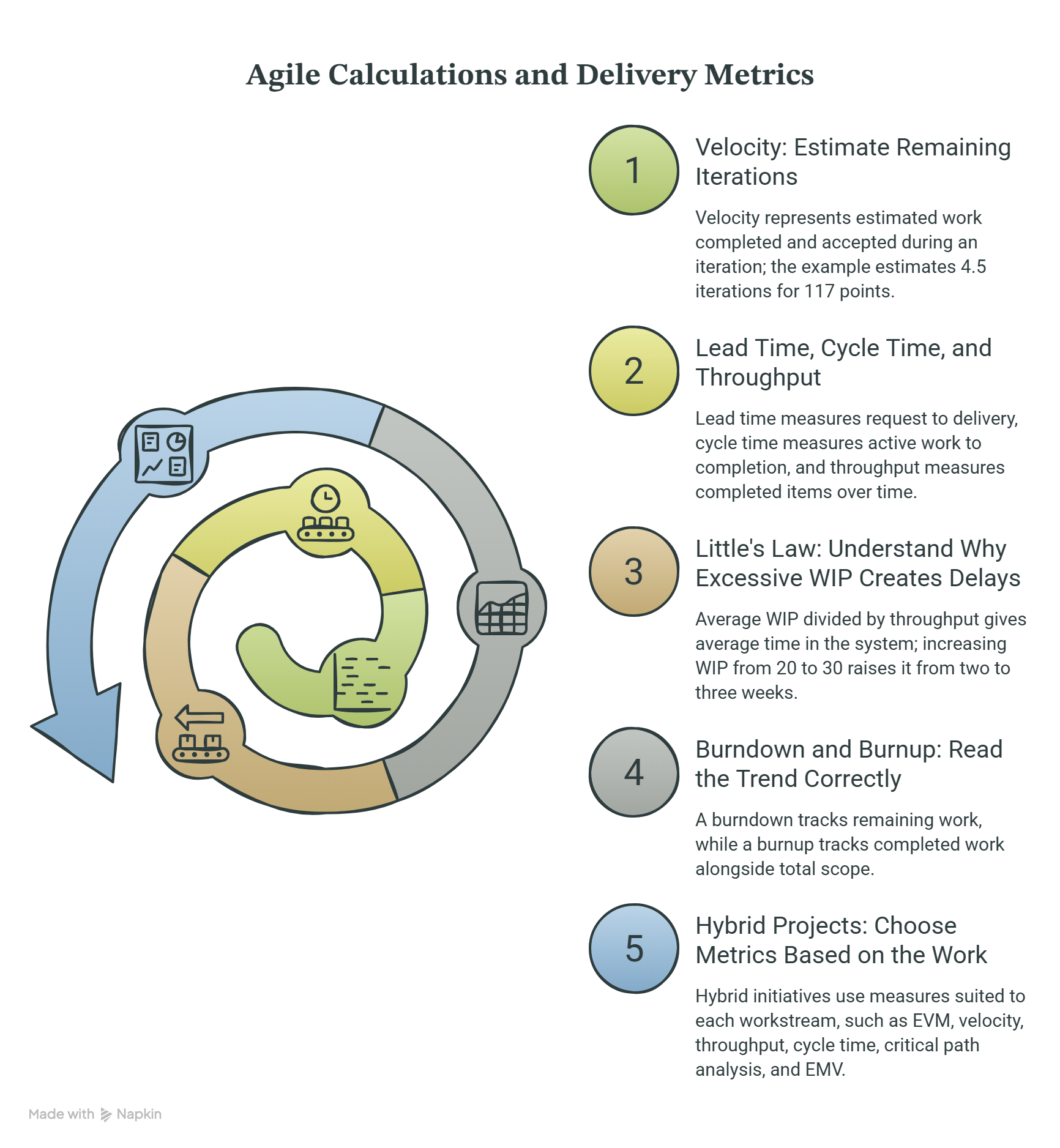
Velocity: Estimate Remaining Iterations
Velocity represents the amount of estimated work a team completes and accepts during an iteration. Story points are one possible unit.
Suppose a team completes:
Sprint 1: 24 story points
Sprint 2: 28 story points
Sprint 3: 26 story points
Average velocity = (24 + 28 + 26) / 3 = 26 points per sprint
If the remaining backlog contains 117 estimated points:
Estimated iterations = 117 / 26 = 4.5
For planning purposes, that suggests approximately five complete sprints, assuming stable capacity, comparable backlog estimates, and similar delivery conditions.
A useful forecast should also consider variability. If upcoming sprints deliver between 22 and 28 points, the team may need approximately five to six sprints, depending on which outcome materializes.
The wider range can produce a more credible commitment than the average alone.
Velocity should never be used to rank unrelated teams because story-point scales are team-specific. This matters in scaled Agile career development, Scrum@Scale coordination, and Agile leadership transitions.
Lead Time, Cycle Time, and Throughput
These three metrics describe different aspects of delivery.
Lead time measures elapsed time from a defined request entry point until delivery.
Cycle time measures elapsed time from the start of active work until completion.
Throughput measures completed items over a defined period.
Suppose a customer requests a feature on Monday, the development team starts it on Thursday, and the feature is delivered the following Tuesday.
Using elapsed calendar time and consistent timestamps:
Lead time: approximately eight days.
Cycle time: approximately five days.
Waiting time before active work: approximately three days.
The difference reveals delays that may exist outside active implementation.
If a team delivers 40 comparable work items over four weeks:
Average throughput = 40 / 4 = 10 items per week
This can help forecast completion when backlog items are consistently defined and the delivery system remains reasonably stable.
Teams can connect these measures with Agile workflow improvement, AI-supported project reporting, project management integrations, and predictive delivery analysis.
Little's Law: Understand Why Excessive WIP Creates Delays
Little's Law describes the relationship between average work in progress, throughput, and time spent in a system.
Average WIP = Average throughput × Average time in system
Suppose a stable delivery process completes 10 items weekly and has 20 items in progress on average.
Average time in system = 20 / 10 = 2 weeks
If average WIP increases to 30 while throughput remains 10 items per week:
Average time in system = 30 / 10 = 3 weeks
The calculation illustrates why continuously starting additional work can increase completion times without increasing output.
Use consistent measurement boundaries. If WIP includes queued and active items, the associated time measure should cover the same system. This relationship also requires reasonable long-run stability.
For PMP scenarios, the appropriate response may involve reducing excessive WIP, removing bottlenecks, or improving flow before adding resources.
This reasoning strengthens Agile team management, scaled delivery systems, operational project leadership, and data-based forecasting.
Burndown and Burnup: Read the Trend Correctly
A burndown chart tracks remaining work over time.
A burnup chart tracks completed work, usually alongside total scope.
For example, suppose a release begins with 120 story points and finishes a sprint with 25 accepted points.
Remaining backlog = 120 − 25 = 95 points
If stakeholders add 20 story points of approved scope, the remaining backlog becomes:
95 + 20 = 115 points
A burndown may show an increase or slower decline despite productive delivery. A burnup chart makes the growth in total scope easier to distinguish from changes in completed work.
Candidates should therefore investigate the cause of a worsening trend before recommending more overtime or replacing the team.
This interpretation supports Agile project management decisions, stakeholder collaboration, and project governance.
Hybrid Projects: Choose Metrics Based on the Work
Hybrid initiatives may combine contractual milestones, fixed budgets, and Agile development.
For example, an enterprise platform rollout may use:
EVM to monitor approved program expenditure.
Velocity to forecast feature development.
Throughput and cycle time to assess support or testing flow.
Critical path analysis for infrastructure and regulatory dependencies.
EMV to compare financially measurable risk responses.
The mistake is combining unlike units without defining their meaning.
Story points do not automatically represent currency. Agile velocity does not directly substitute for schedule SPI. A team can increase velocity while a regulatory approval remains the actual critical-path constraint.
The project manager must select measures appropriate to each workstream and consolidate their implications through program-level oversight, earned value analysis, Agile management techniques, and executive governance.
5. How Should You Memorize PMP Formulas and Solve Questions Under Exam Pressure?
The most reliable preparation method combines formula recognition, calculation practice, interpretation, and timed decision-making.
Candidates frequently spend too much effort memorizing equations in isolation. They then struggle when a question describes the calculation indirectly or includes irrelevant numbers.
A better approach is to organize revision around the decision the formula supports.
This is particularly useful for PMP preparation resources, exam domain practice, common mistake prevention, and exam success strategies.
The Four-Step Calculation Method
Step 1: Identify the requested output.
Look for phrases such as projected final cost, remaining expenditure, expected duration, schedule flexibility, or number of iterations.
These phrases determine the formula family.
Step 2: Identify the data and units.
Separate budget values, actual expenditure, percentages, time estimates, and work units.
Convert percentages into decimals before multiplying. Ensure duration values use compatible units.
Step 3: Select the formula based on the scenario.
For example, if the question says cost inefficiency will continue, consider CPI-based EAC. If a new estimate of remaining work has been prepared, use the bottom-up forecast when appropriate.
Step 4: Check whether the result makes business sense.
A project with negative cost variance and CPI below 1 should generally show financial underperformance.
If a calculation unexpectedly indicates the opposite, check the numerator, denominator, and subtraction order.
Apply this process consistently during EVM calculation practice, PMP study sessions, and exam mistake reviews.
Seven High-Value Formula Memory Rules
Variance uses subtraction; performance indices use division. CV and SV measure differences, while CPI and SPI measure ratios.
For CV and SV, positive usually indicates favorable baseline performance. For CPI and SPI, values above 1 usually indicate favorable performance.
BAC is the authorized budget; EAC is the forecast final cost. ETC is the cost remaining, while VAC is the expected completion variance.
TCPI measures required future efficiency. A TCPI far above current CPI suggests a difficult recovery target.
PERT emphasizes the most likely estimate. Remember the 1:4:1 weighting.
Critical path depends on network logic. The longest calculated path through a network determines its earliest feasible project finish under the assumed constraints.
Agile forecasts depend on stable measurement. Story points, completed work items, calendar time, and currency are different units.
These rules provide a compact foundation for PMP exam readiness, earned value interpretation, Agile learning, and predictive performance management.
A Seven-Day Formula Revision Plan
Day 1: Build the foundation. Learn PV, EV, AC, BAC, CV, SV, CPI, and SPI. Solve calculations using different planned and actual completion percentages.
Day 2: Master financial forecasting. Practice EAC variants, ETC, VAC, and TCPI. Write down the assumption that justifies each forecast.
Day 3: Practice three-point estimation. Calculate PERT, triangular averages, standard deviation, variance, and combined path uncertainty.
Day 4: Solve schedule networks. Complete forward passes, backward passes, critical paths, and float calculations. Include parallel activities and multiple predecessors.
Day 5: Focus on Agile calculations. Practice velocity, backlog forecasts, throughput, cycle time, lead time, and Little's Law. Explain when each calculation is appropriate.
Day 6: Review financial decisions. Practice EMV, ROI, NPV, benefit-cost ratio, and payback. Pay particular attention to cash-flow timing and negative outcomes.
Day 7: Complete mixed timed practice. Combine formula recognition with scenario-based decisions. Review incorrect answers by classifying each mistake as formula selection, data extraction, arithmetic, units, or interpretation.
This schedule can be adapted to your overall PMP study strategy and reinforced through exam mistake analysis, domain-focused revision, and practice-exam preparation.
Use an Error Log Instead of Repeating Entire Question Banks
For each incorrect calculation, record:
The question's requested output.
The formula initially selected.
The correct formula and the reason it applies.
The arithmetic or interpretation error.
A similar question to attempt again.
If three consecutive mistakes involve EAC selection, targeted forecasting practice will usually be more efficient than repeating an entire mixed mock exam.
Track calculation accuracy and time per question separately. A candidate answering correctly but taking several minutes for straightforward problems should practice quicker data extraction.
The objective is reliable application under exam conditions, supported by structured PMP preparation, scenario-based learning, and targeted mistake correction.
6. Frequently Asked Questions About PMP Formulas for 2027–2028
-
Prioritize the EVM family: CV, SV, CPI, SPI, EAC, ETC, VAC, and TCPI. These formulas connect performance measurement with financial forecasting.
Next, focus on PERT, standard deviation, total float, EMV, communication channels, and Agile flow metrics.
The PMP exam assesses broader project management judgment, so formula knowledge should be combined with scenario interpretation. A financially accurate forecast is only valuable when the candidate recognizes the appropriate corrective or governance action.
Candidates can reinforce these concepts through earned value practice, exam preparation resources, exam-domain analysis, and common mistake guidance.
-
Candidates should prepare to recognize and apply the relevant formulas independently. Do not plan your exam strategy around receiving a comprehensive formula reference sheet.
Exam interfaces and available tools can change, so review PMI's current exam-day instructions and your testing provider's calculator and scratch-work rules before the appointment.
Timed practice should emphasize formula selection and numerical interpretation.
The best approach combines PMP study resources, EVM calculation drills, exam success techniques, and mistake prevention.
-
CPI measures cost efficiency: EV / AC.
SPI measures schedule performance relative to planned value: EV / PV.
A CPI of 0.85 indicates financial inefficiency, while an SPI of 1.10 indicates more budgeted value has been earned than scheduled by the status date.
Both metrics can point in different directions simultaneously.
When interpreting them, consider the quality of progress measurement, project phase, and the underlying baseline. Use EVM analysis, predictive forecasting, project governance controls, and project reporting methods.
-
Identify the assumptions about remaining work.
Use BAC / CPI when existing cost efficiency is expected to continue.
Use AC + (BAC − EV) when unfinished work is expected to perform at originally budgeted efficiency.
Use AC + revised ETC when a reliable new estimate of unfinished work has been prepared.
A CPI-and-SPI-adjusted forecast is another scenario-based model when the problem explicitly assumes both indices affect remaining cost.
The correct selection depends on the information given, making EAC forecasting practice, predictive analysis, and PMP exam preparation especially useful.
-
PERT uses the weighted average (O + 4M + P) / 6.
Triangular estimation uses the simple average (O + M + P) / 3.
PERT places greater emphasis on the most likely estimate, while triangular estimation treats all three points equally in the averaging formula.
These estimates provide different planning assumptions rather than guaranteed completion dates.
They are most useful when combined with schedule forecasting, project risk analysis, planning templates, and PMP domain preparation.
-
Agile metrics matter because the PMP framework covers predictive, adaptive, and hybrid delivery approaches.
Candidates should understand how velocity, throughput, lead time, cycle time, WIP, and backlog forecasts support delivery decisions.
However, their meaning depends on context. Higher velocity does not automatically indicate greater business value, and throughput forecasts require a consistent definition of completed work.
Develop these skills through Agile project management, SAFe career guidance, Scrum@Scale learning, and Agile team leadership.
